FERP_publicR
Gregory S Gilbert
2025-04-04
library(tidyverse)
library(ggpubr)
library(grid)
library(knitr)
library(kableExtra)
library(vegan)
library(moments)
Data sets used for analyses of FERP 1, 2, 3 censuses as in
Gilbert, G.S., S.G. Carvill, A.R. Krohn, and A.S. Jones. 2024. Three censuses of a mapped plot in coastal California mixed-evergreen and redwood forest. Forests 15(1), 164; https://doi.org/10.3390/f15010164
South-west coordinate for each 20×20-m quadrat are in quadrat_coords.csv
https://ferp.ucsc.edu/files/2025/04/quadrat_coords.csv
Species names, codes, and attributes are in FERPspecies.csv
https://ferp.ucsc.edu/files/2025/04/FERPspecies.csv
Data from all three censuses are in FERP123_merged_20231029.csv
https://ferp.ucsc.edu/files/2025/04/FERP123merged_20231029.csv
These are accessible from the web URLs below. All other data frames used are subsets or combinations of these data.
Metadata area available at:
https://ferp.ucsc.edu/files/2025/04/Metadata-for-UCSC-FERP123-data-Forests-2024.pdf
## Read in and create the fundamental data frames for use throughout analyses

# Read in data frame with SW coordinate for each quadrat
qc<-read.csv("https://ferp.ucsc.edu/files/2025/04/quadrat_coords.csv")

# Read in data frame with names of all the FERP species
ferpspp<-read.csv("https://ferp.ucsc.edu/files/2025/04/FERPspecies.csv")

# Read in complete data for three censuses
a<-read.csv("https://ferp.ucsc.edu/files/2025/04/FERP123merged_20231029.csv") # read full data

#remove unneeded variables
a<-a[,-which(names(a) %in% c("basalarea1_m2","code6fix","locfix","notes1","notes2","notes3"))]
a$date1<-as.Date(a$date1) #format as Date
a$date2<-as.Date(a$date2) #format as Date
a$date3<-as.Date(a$date3) #format as Date
a$CI12_wk<-as.numeric(a$date2-a$date1)/7 # interval FERP1 to FERP2 census in weeks
a$CI23_wk<-as.numeric(a$date3-a$date2)/7 # interval FERP2 to FERP3 census in weeks

#create separate data frames including only live stems present in each census
f1<-a[a$status1=='living',] # stems alive in FERP1
f2<-a[a$status2=='living',] # stems alive in FERP2
f3<-a[a$status3=='living',] # stems alive in FERP3

# Create data frames for each census with just the largest living stem of each individual
f1_largeststem <- f1 %>% group_by(tag) %>% slice(which.max(dsh1_mm))
f1indiv<-aggregate(f1_largeststem$code6,by=list(f1_largeststem$quadrat),FUN=length)
colnames(f1indiv)<-c("Quadrat","FERP1")

f2_largeststem <- f2 %>% group_by(tag) %>% slice(which.max(dsh2_mm))
f2indiv<-aggregate(f2_largeststem$code6,by=list(f2_largeststem$quadrat),FUN=length)
colnames(f2indiv)<-c("Quadrat","FERP2")

f3_largeststem <- f3 %>% group_by(tag) %>% slice(which.max(dsh3_mm))
f3indiv<-aggregate(f3_largeststem$code6,by=list(f3_largeststem$quadrat),FUN=length)
colnames(f3indiv)<-c("Quadrat","FERP3")
General description of census timing for FERP1 FERP2 FERP3
The first census (FERP1) included only the 6 ha in the southwester portion of the complete FERP; 0 to 200 m East and 0 to 300 m North.
The second census (FERP2) began with that 6 ha, and then expanded the FERP to 400 m East and 400 m North for the full 16 ha.
The third census (FERP3) then included the entire 16 ha.
The censuses proceed generally from West to East.
However, in some cases stems that were missed in the first pass were then re-visited later to get measurements – this can extend the intercensus interval for those stems, or potentially shorten the time if it was measured late in FERP2 and early in FERP3.
FERP1 began 2006-12-08 and ended 2007-09-13.
FERP2 began 2011-09-29 and ended 2015-06-17.
FERP3 began 2017-08-05 and ended 2021-11-29.
FERP2 of the original 6 ha included in FERP1 began 2011-09-29 and ended 2015-02-27.
Of those, 12859 stem observations were completed by 2012-07-06 with an additional 101 by 2015-02-27 to fill in missing data.
FERP3 of the original 6 ha included in FERP1 began 2017-09-28 and ended 2021-10-29.
Of those, 14986 stem observations were completed by 2018-11-12 with an additional 101 by 2021-10-29 to fill in missing data.
Species on the FERP
| Scientific name | Authority | Family | Common name | Origin | Code | Habit |
|---|---|---|---|---|---|---|
| Acer macrophyllum | Pursh | Sapindaceae | Bigleaf maple | Native | ACERMA | tree |
| Adenostoma fasciculatum | Hook. & Arn. | Rosaceae | Chamise | Native | ADENFA | shrub |
| Arbutus menziesii | Pursh | Ericaceae | Pacific madrone | Native | ARBUME | tree |
| Arctostaphylos andersonii | A. Gray | Ericaceae | Santa cruz manzanita | Native | ARCTAN | shrub |
| Arctostaphylos crustacea subsp. crinita | (J.E.Adams) V.T.Parker, M.C.Vasey & J.E.Keeley | Ericaceae | Brittle leaf manzanita | Native | ARCTCR | shrub |
| Baccharis pilularis |
|
Asteraceae | Coyote brush | Native | BACCPI | shrub |
| Ceanothus thyrsiflorus | Eschsch. | Rhamnaceae | Blueblossom | Native | CEANTH | shrub |
| Corylus cornuta subsp. californica | Marshall (A.DC.) A.E.Murray | Betulaceae | Beaked hazelnut | Native | CORYCO | shrub |
| Cotoneaster franchetii | Bois | Rosaceae | Franchet cotoneaster | Intro | COTOFR | shrub |
| Cotoneaster pannosus | Franch. | Rosaceae | Woolly cotoneaster | Intro | COTOPA | shrub |
| Crataegus monogyna | Jacq. | Rosaceae | One-seed hawthorn | Intro | CRATMO | shrub |
| Eriobotrya japonica | (Thunb.) Lindl. | Rosaceae | Loquat | Intro | ERIOJA | tree |
| Eucalyptus globulus | Labill. | Myrtaceae | Blue gum | Intro | EUCAGL | tree |
| Frangula californica | (Eschsch.) A.Gray | Rhamnaceae | California coffeeberry | Native | RHAMCA | shrub |
| Hedera helix | L. | Araliaceae | English ivy | Intro | HEDEHE | liana |
| Heteromeles arbutifolia | (Lindl.) M.Roem | Rosaceae | Toyon | Native | HETEAR | shrub |
| Ilex aquifolium | L. | Aquifoliaceae | English holly | Intro | ILEXAQ | tree |
| Lonicera hispidula | (Lindl.) Douglas ex Torr. & A.Gray | Caprifoliaceae | Pink honeysuckle | Native | LONIHI | liana |
| Morella californica | (Cham.) Wilbur | Myricaceae | California wax myrtle | Native | MORECA | shrub |
| Notholithocarpus densiflorus | (Hook. & Arn.) Manos, C.H. Cannon & S.H.Oh | Fagaceae | Tanoak | Native | LITHDE | tree |
| Pinus attenuata | Lemmon | Pinaceae | Knobcone pine | Native | PINUAT | tree |
| Pinus ponderosa var. pacifica | J.R.Haller & Vivrette | Pinaceae | Pacific ponderosa pine | Native | PINUPO | tree |
| Pseudotsuga menziesii | (Mirb.) Franco | Pinaceae | Douglas fir | Native | PSEUME | tree |
| Pyracantha angustifolia | C.K.Schneid | Rosaceae | Firethorn | Intro | PYRAAN | shrub |
| Quercus agrifolia | Née | Fagaceae | Coast live oak | Native | QUERAG | tree |
| Quercus parvula var. shrevei | (C.H.Mull.) Nixon | Fagaceae | Shreve’s oak | Native | QUERPA | tree |
| Rhododendron occidentale | (Torr. & A.Gray) A.Gray | Ericaceae | Western azalea | Native | RHODOC | shrub |
| Ribes divaricatum | Douglas | Grossulariaceae | Spreading gooseberry | Native | RIBEDI | shrub |
| Salix lasiandra | Benth. | Salicaceae | Pacific willow | Native | SALILA | shrub |
| Sambucus caerulea | Raf. | Vibernaceae | Blue elderberry | Native | SAMBNI | shrub |
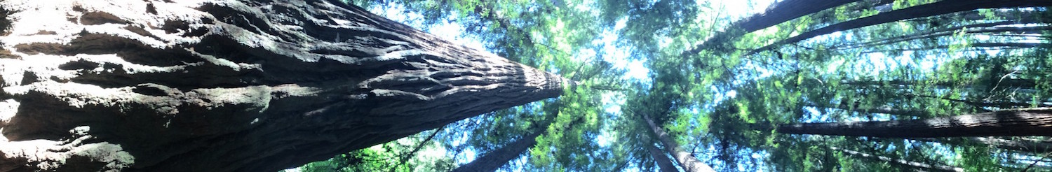
| Sequoia sempervirens | (D.Don) Endl. | Cupressaceae | Coast redwood | Native | SEQUSE | tree |
| Toxicodendron diversilobum | Greene | Anacardiaceae | Poison oak | Native | TOXIDI | liana |
| Umbellularia californica | (Hook. & Arn.) Nutt. | Lauraceae | California bay | Native | UMBECA | tree |
| Vaccinium ovatum | Pursh | Ericaceae | Evergreen huckleberry | Native | VACCOV | shrub |
1Name changes since Gilbert et al. (2010) include VACCOV (from Arctostaphylos tomentosa subsp. crustaceae), LITHDE (from Lithocarpus densiflorus), RHAMCA (from Rhamnus califonica), and SAMBNI (from Sambucus nigra subsp. caerulea). Original 6-letter codes are retained for continuity. The family of SAMBNI also changed from Caprifoliaceae to Vibernaceae.
Number of individuals, stems, and species in each census
Individuals are represented by the largest living stem at that census.
These are data used to create Table 2.
FERP1 included 8185 live individuals and 11646 stems of 31 species in 6 ha.
FERP2 included 26084 live individuals and 39821 stems of 34 species in 16 ha.
FERP3 included 24939 live individuals and 36849 stems of 33 species in 16 ha.
FERP2 of the original 6 ha included in FERP1 included 8273 live individuals and 11954 stems of 30 species in 6 ha.
FERP3 of the original 6 ha included in FERP1 included 6949 live individuals and 10344 stems of 28 species in 6 ha.
For all censuses combined, this represents 48556 stems from 31206 individuals that have been mapped and observed.
(Note: the following have unresolvable values for dsh2 and dsh3 and are removed from analyses of growth, but are retained for other summaries: SEQUSE 16482 1; SEQUSE 26772 1; SEQUSE 20864 1; QUERPA 22433 1 )
Map plot and size histogram of a species from FERP3 census
Options for species codes are as given in table above: ACERMA ADENFA ARBUME ARCTAN ARCTCR BACCPI CEANTH CORYCO COTOFR COTOPA CRATMO ERIOJA EUCAGL RHAMCA HEDEHE HETEAR ILEXAQ LONIHI MORECA LITHDE PINUAT PINUPO PSEUME PYRAAN QUERAG QUERPA RHODOC RIBEDI SALILA SAMBNI SEQUSE TOXID UMBECA VACCOV
Set the species code of interest
species<-"SEQUSE"
plot(f3$east_m[f3$code6==species],f3$north_m[f3$code6==species],asp=1,ylab=NA,xlab=NA,
     las=1, xlim=c(0,400),ylim=c(0,400),main=paste(species,"FERP3"),
     cex=sqrt(f3$dsh3_mm[f3$code6==species]/500),col="black")
abline(h=seq(0,400,20),lty=2,col="grey80"); abline(v=seq(0,400,20),lty=2,col="grey80")
st<-f3[f3$code6==species,]
hist(st$dsh3_mm[st$code6==species]/10,breaks=seq(0,floor(max(st$dsh3_mm,na.rm=T)/10+5),5),
las=1, main=paste(species,"FERP3"), ylim=c(0,200),col="blue",xlab="Diameter standard height (mm)",ylab="Number of stems")Map plot of a species from FERP2 census
species<-"QUERAG"
plot(f2$east_m[f2$code6==species],f2$north_m[f2$code6==species],asp=1,ylab=NA,xlab=NA,
     las=1, xlim=c(0,400),ylim=c(0,400),main=paste(species,"FERP2"),
     cex=sqrt(f2$dsh2_mm[f2$code6==species]/500),col="black")
abline(h=seq(0,400,20),lty=2,col="grey80"); abline(v=seq(0,400,20),lty=2,col="grey80")
st<-f2[f2$code6==species,]
hist(st$dsh2_mm[st$code6==species]/10,breaks=seq(0,floor(max(st$dsh2_mm,na.rm=T)/10+5),5),
las=1, main=paste(species,"FERP2"), ylim=c(0,200),col="blue",xlab="Diameter standard height (mm)",ylab="Number of stems")